Example: Heatflow in one dimension
This is an example of efficient prototyping of recurrences applied to a simple partial differential equation.
The 1-dimensional heat flow equation describes the heat distribution u(x,t) in
a one-dimensional object along the x-axis at time t. Alpha is a physical constant describing the heat transfusion properties of the object.

![]()
![]()
![]()

h(n) =
  if(right_boundary(n) or left_boundary(n)
    then h(d(n,2))
  else
    s*h(d(n,1))
  + (1-2*s)*h(d(n,2))
  + s*h((d(n,3)
x int * t int
rather than in real coordinates. The opposite of the stencil becomes

![]()
![]()
Heatflow computation
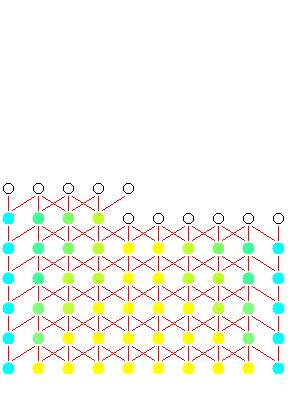
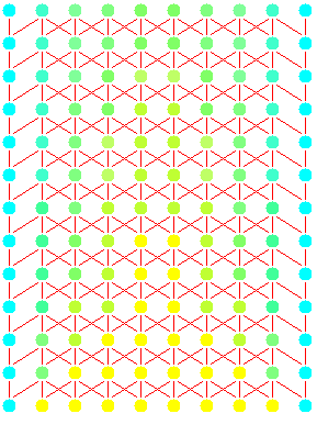
The following is a sequence of snapshots of the actual computation generated by the compiler. The temperature has been encoded using colours. Initially the rod is hot (yellow), with a constant cold temperature (blue) being applied at the ends. During time the rod cools off from the edges (hues of green).After sending initial values:
 |
|
While computing:
 |
|
Complete computation:
 |
|
You can watch an animated demo of this if your browser supports Java.
In the parallel case all nodes at the same timestep would be computed simultaneously. An animated demo of this has also been prepared as a Java applet.
Heatflow result
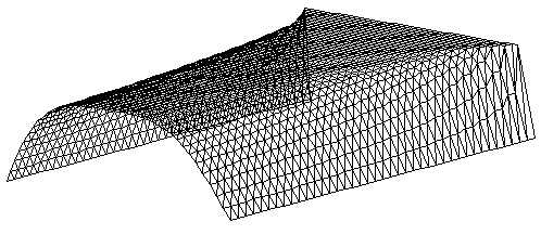
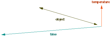
Below the temperature of the object has been plotted against time in a wireframe image. You may view this as a rotatable image written in Java.


This was an example of efficient prototyping of recurrences.
© 1997 Magne Haveraaen, University of Bergen, Norway.
